In the realm of Data Analysis and Digital Marketing, we frequently encounter scenarios where we must extract numerical values that follow specific symbols or special characters like “$” or “=” within a provided string. This need becomes more intricate when the said symbols appear multiple times within the string. In such cases, our objective is to pinpoint the second occurrence of the designated symbol and subsequently capture the corresponding substring or numeric value, thereby populating a distinct column with this information. In this post we discuss about 3 Steps to Get Substring after nth Occurance in Microsoft Excel.
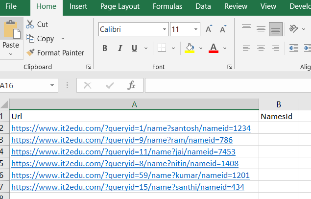
See the below image, in this Image Column A has Url’s and Column B is empty. No we need data in B. The expected data in B column is last digits after “=” symbol.


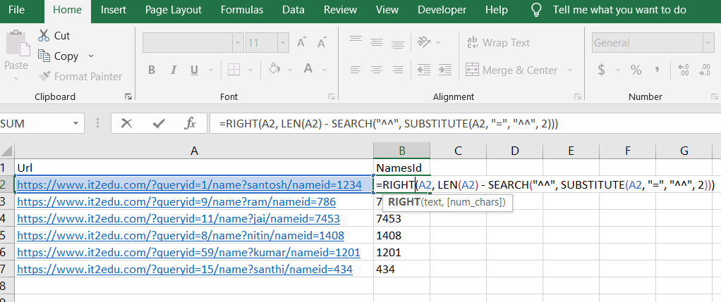
To get the data in column B, use a formula in column B2.
=RIGHT(A2, LEN(A2) - SEARCH("^^", SUBSTITUTE(A2, "=", "^^", 2)))
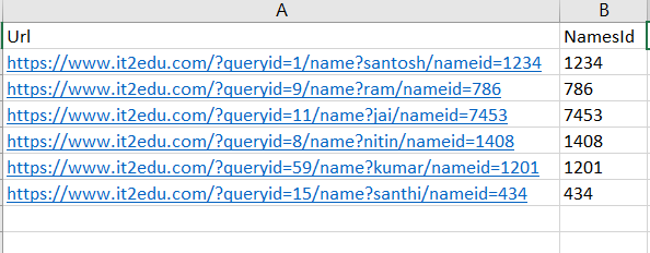
Now we get the value as expected in column B and drag upto end.

explanation of the formula:
To extract the number after the second occurrence of the equal symbol (=) or any special symbol in a string using the RIGHT, SEARCH, and LEN functions in Excel, you can use a combination of these functions. Let’s assume your string is in cell A1, and you want to extract the number after the second equal symbol in another cell (let’s say B1). Here’s how you can do it:
To extract the number after the second occurrence of the equal symbol (=) in a string using the RIGHT, SEARCH, and LEN functions in Excel, you can use a combination of these functions. Let’s assume your string is in cell A1, and you want to extract the number after the second equal symbol in another cell (let’s say B1). Here’s how you can do it:
Explanation of the formula:
SUBSTITUTE(A1, “=”, “^^”, 2): This substitutes the second occurrence of “=” with “^^” in the string. This avoids confusion since “^” is a special character used to escape other characters.
SEARCH(“^^”, SUBSTITUTE(A1, “=”, “^^”, 2)): This finds the position of the second occurrence of “^^” in the modified string.
LEN(A1) – SEARCH(“^^”, SUBSTITUTE(A1, “=”, “^^”, 2)): This calculates the length of the portion of the string after the second “=”.
RIGHT(A1, LEN(A1) – SEARCH(“^^”, SUBSTITUTE(A1, “=”, “^^”, 2))): This extracts the portion of the string after the second “=”.
Other articles on Data Analytics or Power Bi is here.
Microsoft Excel functions here.
 IT2EDU Empowering Education Through Technology
